Task Options
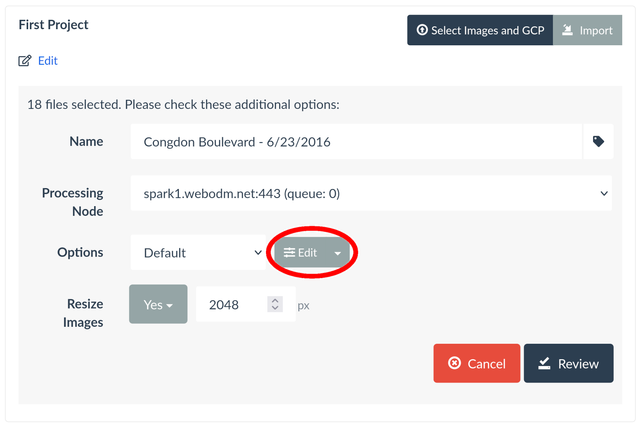
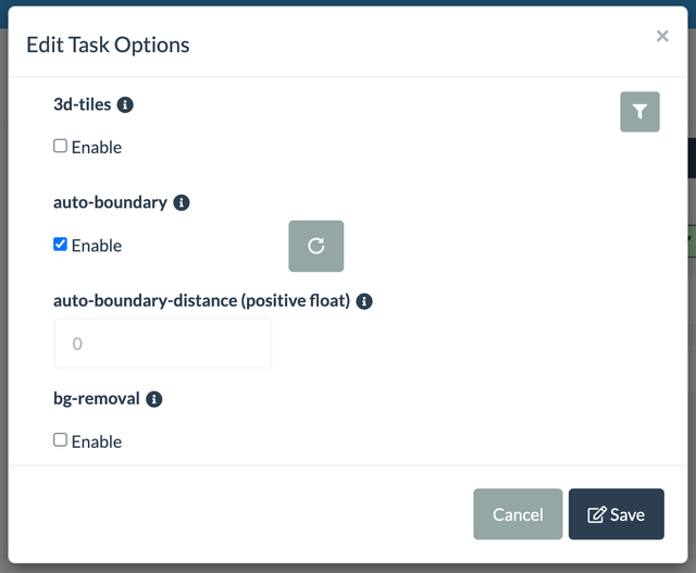
When creating a task, press the Edit button next to the Options field:
In general, it's a good idea to begin with the default settings, which usually work well for most datasets, and make adjustments as necessary.
3d-tiles
3D Tiles are a format specification for visualizing and interacting with 3D geospatial content. You can view these files using software like Cesium. WebODM Lightning can generate point clouds and textured 3D models in 3D Tiles format. Turn on this option to generate them.
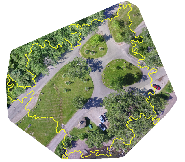
auto-boundary
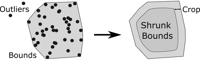
Automatically calculates a 2D polygon that encloses the camera pose locations. This polygon is subsequently employed as an input for the boundary option. The polygon is generated using a convex hull and it's adjusted with a distance buffer that scales with the flight altitude, with higher altitudes leading to larger buffers.

auto-boundary-distance
Manually adjust the distance buffer value (in meters) for auto-boundary.
bg-removal
Utilizes artificial intelligence techniques to automatically create image masks for background removal. This is particularly valuable for generating 3D models of individual objects. However, it may not work well in aerial scenes.
See also sky-removal.
boundary
Specify a single polygon boundary in GeoJSON format, which is used to define the reconstruction area.
GeoJSON polygons can be created using software like QGIS or online tools like geojson.io. Additionally, you can automatically generate them using the auto-boundary option.
If the crop option is set to zero, the boundary polygon can also serve as the crop area for DEMs and orthophotos.
camera-lens
Digital camera sensors quantify the incoming light. Prior to reaching the sensor, light traverses through a camera lens. Lenses introduce different degrees of distortion into photos, with the specific type of distortion determined by the lens shape. This distortion can range from pronounced, such as in fisheye or wide-angle lenses, to more subtle in the case of perspective lenses. It's essential to recognize that some level of distortion is invariably present.
WebODM Lightning offers support for multiple lens models and automatically selects the most suitable one by considering the information available in the EXIF1 and XMP2 tags of the images. Nevertheless, there are instances where such information is absent. In these cases, if you encounter difficulties when processing images captured with a fisheye lens, it's advisable to manually designate either fisheye or fisheye_opencv as the camera-lens option. As a general guideline, when your input images exhibit noticeable distortion, it's a prudent approach to manually configure this option with the appropriate value.
| Value | Images | Description |
|---|---|---|
| auto | Normal | Defaults to brown, unless the XMP tag GPano:ProjectionType or Camera:ModelType contains a value from this table |
| perspective | Normal | Handles radial distortion |
| brown | Normal | Handles radial, tangential, and principal point distortions |
| fisheye | Ultra wide-angle | Handles radial distortion |
| fisheye_opencv | Ultra wide-angle | Handles radial distortion, tangential, and principal point distortions |
| spherical | 360 | Handles spherical projection for 360 images |
| equirectangular | 360 | Same as spherical (legacy name) |
| dual | Ultra wide-angle / Normal | Handles radial distortion from sensors that can capture both fisheye and perspective images, transitioning from one to the other. |
Please be aware that utilizing this option applies the same camera lens model to all images, even if they originate from different cameras. To apply distinct models for different cameras, it's necessary to ensure that the images have the appropriate XMP tags set.
cameras
By default WebODM Lightning estimates the camera model's distortion parameters from the input images. This option allows you to choose a precomputed set of parameters instead from another task. You can do this by providing a cameras.json file, which is generated after processing a dataset and can be downloaded from the cloud interface by clicking Download → Camera Parameters. This feature can be helpful in improving the accuracy of certain datasets, especially those that didn't follow good image capture guidelines.
crop
The crop area for orthophotos and DEMs is calculated from the point cloud, first by defining a convex hull around the points and then shrinking it by crop amount (in meters).
This option can be set to zero to skip cropping.
One can also set the boundary option and set this option to zero to manually define the crop area.
crs
Specify the Coordinate Reference System (CRS) to use for processing. It can be set to one of the following values:
| Value | Example | Description |
|---|---|---|
utm (default) | utm | Use the closest UTM zone based on the images' GPS. |
gcp | gcp | Use the same CRS as the GCPs. If no GCP file is provided, reverts to utm. |
EPSG:code | EPSG:32616 | Custom EPSG code definition. |
EPSG:code+vertical | EPSG:6527+6360 | NAD83(2011) / New Jersey (ftUS) (6527) + NAVD88 height (ftUS) (6360). Geoid automatically selected. |
EPSG:code+vertical(geoid) | EPSG:6527+6360(GEOID18) | Explicitly defines the geoid model to use. |
PROJ definition | +proj=utm +zone=16 +datum=WGS84 +units=m +no_defs +type=crs | Legacy and not recommended, but can be useful if an EPSG code does not exist. |
See also the list of geoids.
dem-euclidean-map
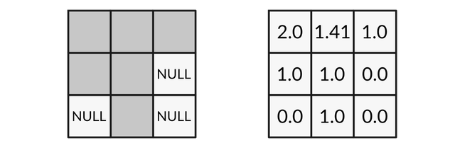
An Euclidean map is a georeferenced image created from Digital Elevation Models (DEMs) before filling any gaps. In this image, each pixel represents the geometric distance to the nearest void, null, or NODATA pixel. It serves as a visual indicator of how far a value in the DEM is from an area with no data. This is valuable when you want to distinguish areas in the DEM that are based on actual point cloud values from those filled with interpolation.
In the Euclidean map, every pixel with a value of zero indicates that the corresponding location in the DEM was filled using interpolation, as the distance from a NODATA pixel to itself is zero. You can generate this map by turning on this option.
The resulting map will be available from Download → All Assets in the odm_dem folder.
dem-resolution
This option specifies the output resolution of DEMs in cm / pixel.

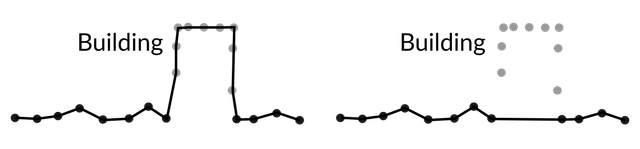
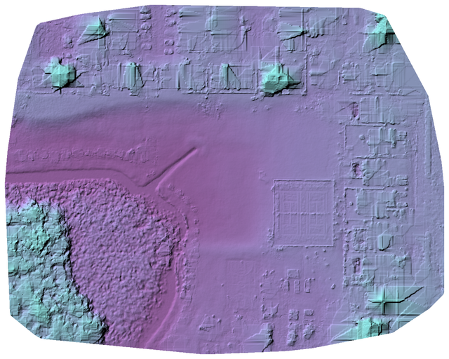
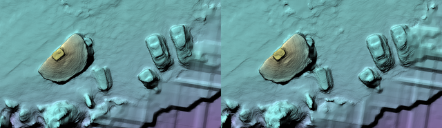
dsm
This option creates a digital surface model (DSM). DSMs are created by identifying the highest elevation values in a point cloud, which includes terrain and various structures like buildings and trees. When two points coincide, only the tallest point is considered.
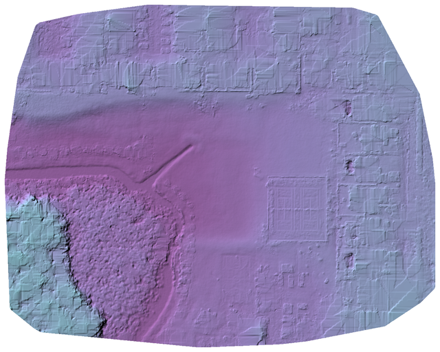
dtm
This option creates a digital terrain model (DTM). DTMs are created by applying a hybrid method that combines a simple morphological filter3 (SMRF) with artificial intelligence. Enabling this option also activates the pc-classify feature. Non-ground points are removed before DTM calculation. For additional details refer to the pc-classify option.
end-with
Instead of processing the entire photogrammetry pipeline, the pipeline will stop the execution at the chosen step.
| Option | Stage |
|---|---|
| dataset | Load Dataset |
| split | Split |
| merge | Merge |
| opensfm | Structure From Motion |
| openmvs | Multi View Stereo |
| odm_filterpoints | Point Filtering |
| odm_meshing | Meshing |
| mvs_texturing | Texturing |
| odm_georeferencing | Georeferencing |
| odm_dem | DEM |
| odm_orthophoto | Orthophoto |
| odm_report | Report |
| odm_postprocess | Postprocess |
fast-orthophoto
For flat areas (agriculture fields), this option can save some substantial computation time by not requiring the construction of the dense point cloud used for orthorectification. This option does not work well in urban scenes due to excessive relief displacement artifacts.
feature-quality
The photogrammetry process starts by identifying points of interest (features) from the input images. To expedite this, extraction is performed on a scaled-down version of the input images, determined by a scaling factor.
| Option | Factor |
|---|---|
| high | 1/2 (default) |
| medium | 1/4 |
| low | 1/8 |
| lowest | 1/16 |
For example, choosing medium uses 1/4 of the original image size. The default value works for most cases, without affecting image sizes or orthophoto resolution. Sometimes, decreasing this value can be helpful in forest areas that lack sufficient overlap.
feature-type
WebODM Lightning provides multiple algorithms for extracting image features. For the most consistent and reliable results, I recommend to use the default dspsift algorithm. However, in specific scenes or situations, you may benefit from using alternative algorithms. Refer to the table below.
| Option | Description |
|---|---|
| sift | General-purpose, works well in most cases4 |
| dspsift | General-purpose, slower but generally more accurate than sift. Performs better in scenes with low overlap or vegetation5 |
| akaze | General-purpose, can perform better on scenes with fewer objects of interest (e.g. forests, vegetation)6 |
| hahog | General-purpose, similar to sift. |
| orb | Fast, but does not work well with images that have scale variations (images taken at varying altitudes)7 |
force-gps
When a GCP file is utilized, the default behavior is to disregard all GPS data, relying solely on the GCP file for georeferencing. The underlying assumption is that GCP data is more accurate than GPS. However, if the GPS data is highly accurate (e.g., with RTK8 correction), enabling this option directs the program to use both GCP and GPS data for georeferencing.
gps-accuracy
GPS data has a certain level of accuracy. This value is used to specify how much GPS data should be constrained during the photogrammetry process.
Typically, accuracy information is obtainable from XMP tags in the images. WebODM Lightning uses twice the number indicated in any of the following tags (to account for underestimation):
- drone-dji::RtkStdLon
- drone-dji::RtkStdLat
- drone-dji::RtkStdHgt
- Camera::GPSXYAccuracy
- GPSXYAccuracy
- Camera::GPSZAccuracy
- GPSZAccuracy
If multiple tags are present, the maximum value is used. If no tags are available, the default is 10 meters.
gps-z-offset
Adds a GPS offset in meters to all GPS measurements in the vertical (Z) axis:
GPS Z = GPS Z + offset
This is applied to all images and does not affect GCPs. It can be used to adjust incorrect elevation readings. By default no adjustments are made.
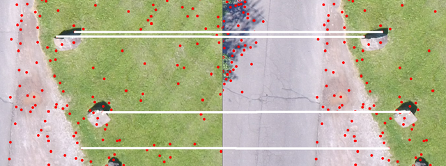
matcher-neighbors
During reconstruction image pairs are matched by identifying common features. The brute-force approach compares each image with every other, resulting in exhaustive but slow searching. For a 100-image dataset, it would require numerous comparisons.
print(100 * (100 - 1)) # <-- 9900 comparisons
To enhance efficiency, the program employs optimizations. The concept is that for datasets gathered uniformly, most images are paired with nearby ones. Using GPS data, the program quickly approximates which images are adjacent and excludes distant ones. This process is called preemptive matching.
WebODM Lightning applies a graph connectivity approach for preemptive matching. It uses GPS locations to link images with edges through Delaunay triangulation9. If two images share an edge, they form a pair. To generate more pairs, the method shuffles GPS locations to create multiple graphs (a total of 50). All pairs from these graphs are considered for further matching. This method is always enabled (if GPS locations are available).
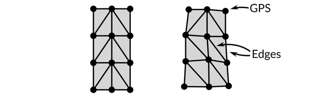
In addition to graph matching, WebODM Lightning also applies a nearest neighbor matching method that focuses on the nearest neighbors of each image. By default this option is set to 8.
You can turn off this method by setting it to 0. If no GPS information is available, this method is disabled.
matcher-order
Like matcher-neighbors, this option decreases the number of candidate pairs for matching based on the sequential order of image filenames. For instance, if you have 3 images sorted by filename:
- 1.JPG
- 2.JPG
- 3.JPG
With this option set to 1, the program will evaluate matches between:
- 1.JPG and 2.JPG
- 2.JPG and 3.JPG
This is because the "distance" between these image pairs in the list is 1. 1.JPG and 3.JPG have a distance of 2, so this pair will be excluded from matching.
This option determines the maximum distance between image filenames for them to be considered a matching pair. It is exclusively useful for datasets without GPS information, particularly for expediting the processing of sequentially ordered images, like frames extracted from videos.
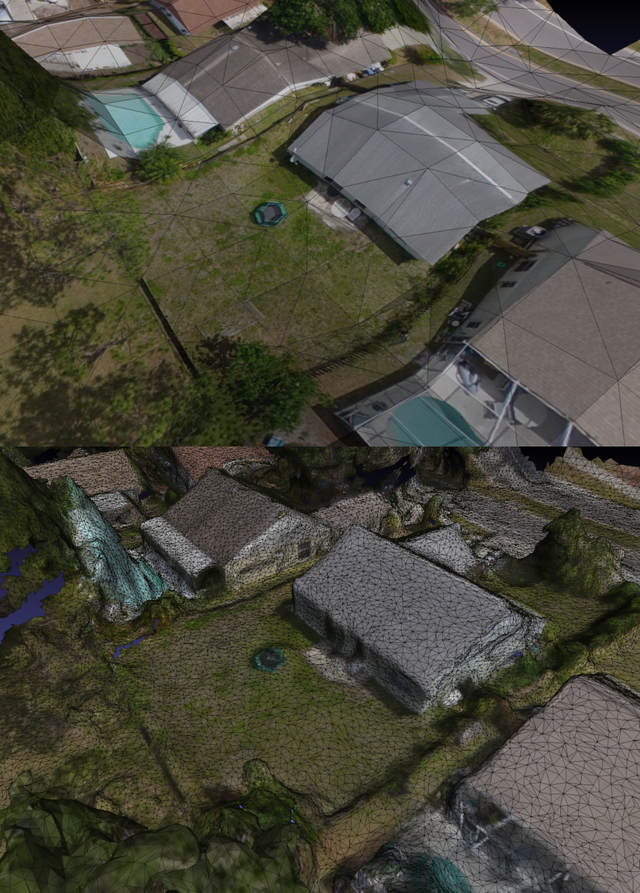
mesh-octree-depth
Controls the quality of the 3D textured models. A higher value results in a finer model. However, this comes at the cost of significantly increased processing time. The default value of 11 is suitable for most scenarios. Lower values (6-8) can be sufficient in flat areas, while setting it higher (12) can improve results in urban areas. When raising this option, consider increasing mesh-size as finer meshes require more triangles.
mesh-size
WebODM Lightning automatically simplifies the textured 3D models by limiting their triangle count. A high triangle count prolongs subsequent processing steps. A low count can reduce model quality, while increasing it can enhance results, especially in urban areas requiring fine building details.
min-num-features
This option controls the minimum number of features detected in each image, increasing the potential for finding matches.
Increase this option when mapping areas with few discernible features, like forests.
optimize-disk-space
This option is always turned on. No need to worry about it.
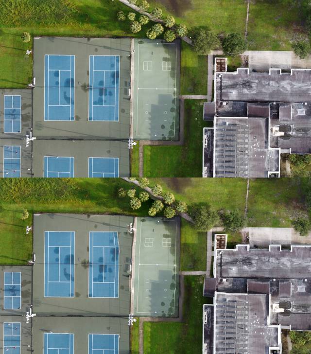
orthophoto-cutline
Enabling this option results in the program creating a cutline, which is a polygon within the crop area of the orthophoto that aims to trace feature edges.
The resulting cutline can be downloaded from the cloud interface by clicking Download → All Assets (odm_orthophoto/cutline.gpkg).
orthophoto-resolution
This option specifies the output resolution of the orthophoto in cm / pixel.
See also dem-resolution.
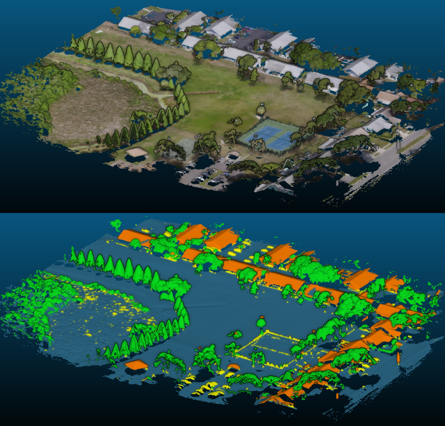
pc-classify
Points in a point cloud can be assigned classification values10 to indicate if they belong to the terrain (ground), a building, a tree (vegetation), or other categories. By default, all points are labeled as unclassified, and the software doesn't assign specific labels to points. Enabling this option utilizes a Simple Morphological Filter3 (SMRF) to identify and classify terrain points as ground. An AI classifier11 is then applied to the remaining (non-ground) points to recognize vegetation, buildings, and other structures. This process results in a classified point cloud.
| Option | Description |
|---|---|
| smrf-scalar | This parameter makes the threshold dependent on the slope. To enhance results, consider slightly decreasing this value when raising the smrf-threshold, and vice versa.. |
| smrf-slope | Set this parameter to the steepest common terrain slope, represented as the ratio of elevation change to horizontal distance change (e.g., 1.5 meters over 10 meters is 1.5 / 10 = 0.15). Increase it for terrains with significant slope variation, like hills and mountains, and reduce it for flat areas. For optimal results, it should be above 0.1 but not exceed 1.2. |
| smrf-threshold | Defines the minimum height (in meters) of non-ground objects. For instance, a setting of 5 meters is suitable for identifying buildings but may not suffice for recognizing cars. To identify cars, lower the value to 2 or even 1.5 meters (the average car height). This parameter significantly influences results. |
| smrf-window | Set this to the size of the largest non-ground feature in meters. If the scene primarily consists of small objects like trees, reduce this value. If there are larger objects like buildings, increase it. It's advisable to maintain a value above 10 meters. |
SMRF has limitations, including occasional misclassification of buildings or trees as ground points (type II errors).
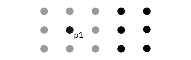
pc-filter
Noise from the point cloud can be partially removed using a combination of statistical and visibility filtering. This option sets the standard deviation threshold value for the statistical filter. In this context standard deviation is a measure of how spread out points are relative to their neighbors. The filter looks at the closest 16 neighbors for each point and computes their standard deviations, which gives a measure of how far each point deviates from the average distance to each other point. If a point is found to be too far away relative to its neighbors, thus having a standard deviation higher than the threshold, the point is labeled as an outlier.
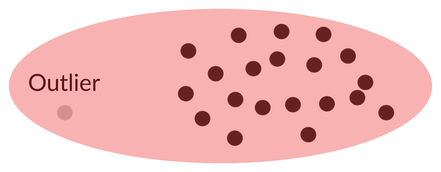
Adjusting this value too high retains noisy points, and setting it too low may eliminate valid ones. You can disable filtering by setting this option to zero.
pc-quality
This option affects the density of the point cloud. Higher values use higher resolution images according to a scale factor:
| Option | Scaling Factor |
|---|---|
| high | 1/4 |
| medium | 1/8 |
| low | 1/16 |
| lowest | 1/32 |
Different image dimensions also correspond to a multiplier value:
| Largest Image Dimension (megapixels) | Multiplier |
|---|---|
| < 6 | 2 |
| 6 - 42 | 1 |
| > 42 | 1/2 |
The actual resolution of the images used for point cloud estimation is then calculated with:
resolution = max(320, max_image_dimension * scaling_factor * multiplier)
For example, in a dataset with 4000x3000 (12 megapixels) images, setting this option to high will use images scaled to 1000 pixels for computing a point cloud:
image = (4000,3000)
max_image_dimension = max(image) # <-- 4000
megapixels = image[0]*image[1]/1000000 # <-- 12
multiplier = 1 # From table
scaling_factor = 1/4 # pc-quality: high
print(max(320, max_image_dimension * scaling_factor * multiplier)) # <-- 1000 pixels
pc-sample
This option imposes an upper limit on the density of the dense point cloud, defined as a radius in meters that ensures no two points are closer than the specified value. For instance, a setting of 0.05 ensures points are at least 5 centimeter (0.05 meters) apart. By default all points are kept.
pc-skip-geometric
A geometric refinement process is used to improve the point cloud. This process can take some time and can be skipped by using this option.
primary-band
This option selects the band name (Red, Blue, Green, NIR, etc.) for reconstructing multispectral datasets. The chosen band name must match the Camera::BandName EXIF1 tag. Only the images associated with this band will be utilized for 3D reconstruction.
By setting it to auto (the default), the band will be automatically selected.
radiometric-calibration
Radiometric calibration converts pixel values (digital numbers) into reflectance. WebODM Lightning can automate radiometric calibration and compute reflectance and temperature values for various sensors12.
| Option | Description |
|---|---|
| none | No radiometric calibration (digital number outputs) |
| camera | Applies black level, vignetting, gain, and exposure corrections based on information from the EXIF tags. Additionally, computes absolute temperature values when applicable |
| camera+sun | Same as camera, but also applies corrections from a downwelling light sensor (DLS) when available |
report-units
Set the units of the quality report (PDF).
| Option | Description |
|---|---|
| auto | Use the same units as those of the selected coordinate reference system |
| m | Metric units |
| ft | Imperial units |
| US survey foot | Imperial units (US) |
rerun-from
This option cannot be used. Don't worry about it.
rolling-shutter
Enables rolling shutter correction to enhance reconstruction accuracy in datasets captured with rolling shutter sensors. If GPS information is present in the input images, and the dataset was captured with a single camera, WebODM Lightning can correct for rolling shutter distortion by initially estimating the aircraft's velocity at the time each picture was taken. Some cameras store velocity information in the EXIF/XMP tags of the images (SpeedX, SpeedY, and SpeedZ), which provides the most reliable estimate. In the absence of these tags, velocity is estimated based on the time and positional differences between consecutive images.
speed = (position_2 - position_1) / (time_2 - time_1)
The accuracy of the formula mentioned above can be compromised in situations where the drone is stationary while capturing a picture, as it assumes continuous motion and sequential image capture. In such cases, the calculation may yield incorrect estimates, potentially degrading results. However, as long as most images can be assigned accurate velocity estimates, rolling shutter correction can still be effective, even if a few images have incorrect estimates.
Once the velocities are estimated, the program searches a database to retrieve the rolling shutter readout time for the camera sensor. This readout time represents the duration (in milliseconds) required for the sensor to capture an image. In cases where your camera is not listed in the database, a warning will appear in the task output:
[WARNING] Rolling shutter readout time for "make model" is not in
the database, using default of 30ms which might be incorrect.
With known camera velocities and sensor readout times, the correction is applied by shifting image features based on these factors. Subsequently, the reconstruction is repeated, effectively doubling the processing time but enhancing accuracy in datasets influenced by rolling shutter distortions.
You can estimate the correct sensor value by creating a cost-effective calibration device using an Arduino. Detailed instructions are available at github.com/OpenDroneMap/RSCalibration.
rolling-shutter-readout
Overrides the default sensor readout time value used for rolling shutter correction.
sfm-algorithm
There are three methods to reconstruct a scene:
| Option | Description |
|---|---|
| incremental | a general-purpose approach suitable for all scenes. It supports multiple cameras and adds them to the reconstruction incrementally, ensuring high reliability. |
| triangulation | If gimbal angles and GPS information are available, camera positions are initialized from those values in a single step and then iteratively improved. This method can yield better results and may be slightly faster than incremental. However, it's experimental and may not work with all camera types. |
| planar | For flat scenes, like a farm field, captured with a single camera at a constant altitude and a downward-facing view (nadir), this option is recommended. It processes 5-10 times faster than the incremental method and is compatible with multispectral datasets. |
skip-3dmodel
If a user only needs an orthophoto, there's no need to create a complete 3D model. This option saves time by skipping the steps for generating a 3D model. Instead, it creates a 2.5D model, where elevation is extruded from the ground plane. While not a full 3D model, it works effectively for rendering orthophotos, although it can't accurately represent objects like overhangs.
See also use-3dmesh.
skip-band-alignment
When capturing multispectral images, the sensors for each band are often slightly misaligned, causing small misalignments between the image bands. ODM automatically aligns these bands as part of its multispectral processing. If manual alignment has already been done using other software, you can disable the automatic alignment using this option.
skip-orthophoto
If you don't require an orthophoto, this option can save you time by skipping the orthophoto generation step.
skip-report
If you don't require a PDF report, this option can save you some time by skipping the report generation step.
sky-removal
Utilizes AI methods to automatically create image masks for sky removal. This is beneficial for datasets that include sky portions, especially in cases where oblique images are used for 3D structure capture. Sky areas can introduce noise in the 3D model, and this option helps in its reduction.
smrf-scalar
Sets the scalar variable for SMRF. See pc-classify.
smrf-slope
Sets the slope variable for SMRF. See pc-classify.
smrf-threshold
Sets the threshold variable for SMRF. See pc-classify.
smrf-window
Sets the window variable for SMRF. See pc-classify.
texturing-data-term
The textured 3D model is colored using a selection of the input photos. Which photos are assigned to which triangle in the mesh depend on the choice of the data term strategy:
| Option | Description |
|---|---|
area (default) | Prioritizes the area of each back-projected triangle to the camera frame. Picks the photo that covers the largest area (offers the most pixels). |
gmi | Prioritizes based on a gradient magnitude image, which picks the photo that provide the sharpest pixels. |
nadir | Prioritizes based on camera angle and favors nadir (down-facing) photos. |
texturing-regularization
Images with significant color variations caused by differences in illumination and exposure need to be merged using a global optimization process. The amount of correction is controlled by a factor which can be either:
| Option | Description |
|---|---|
fixed (default) | Uses a fixed, static value. This works generally well, but can sometimes fail if a dataset contains several over-exposed or under-exposed images, causing large gradients to appear in the result. |
dynamic | Dynamically sets the amount of color correction based on the input images. This can improve color balance and fix problems with large gradients. |
See also texturing-skip-global-seam-leveling
texturing-single-material
The 3D models created by WebODM Lightning are in the Wavefront OBJ13 format. This format supports storing color information across multiple image files (textures). Each texture in the model is linked to a "material." WebODM Lightning typically uses multiple materials and textures when generating OBJ files by default. However, some software may have issues opening OBJs with multiple materials, or performing certain operations on meshes with multiple materials, which can be complex. This is especially true when editing the mesh in programs like Blender14.
Enabling this option will produce an OBJ file with a single material.
texturing-skip-global-seam-leveling
Images with significant color variations caused by differences in illumination and exposure need to be merged using a global optimization process. This process slightly affects reflectance/temperature values when processing multispectral datasets and it might be desirable to enable this option to turn it off.
See also texturing-regularization
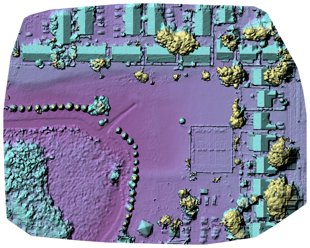
tiles
This option creates static TMS15 tiles for orthophotos and DEMs, ideal for hosting and sharing maps on websites. These tiles work seamlessly with various viewers, like Leaflet16. DEM tiles are produced with a colored hillshade style and can be downloaded from the cloud interface by clicking on the Download button.
use-3dmesh
By default, a 2.5D textured mesh is used for orthophoto rendering, which usually works well for most aerial datasets. However, it may yield suboptimal results, especially when nadir images (images with the camera pointed straight or nearly straight at the ground) are missing. Furthermore, for specific scenes like single building orbits with oblique images, a 2.5D mesh may not perform well.
This option instructs the program to utilize the full 3D model for orthophoto generation while skipping the creation of the 2.5D model. For additional information, see skip-3dmodel.
use-exif
When a GCP file is uploaded with a dataset, it is always used for georeferencing. Enabling this option causes the program to disregard the GCP file and rely on location information from the images' EXIF1 tags instead.
use-fixed-camera-params
Camera internal parameters are estimated and refined during reconstruction. Poor image capture practices can lead to incorrect estimations and a "doming" effect. Enabling this option keeps camera parameters fixed, potentially improving results when images have little geometric distortion.
This option will not magically fix problems associated with poor image captures.
video-limit
WebODM Lightning can process video files (.mp4, .mov, .lrv, and .ts) by extracting image frames at regular intervals. The program automatically filters out blurry and dark frames.
For DJI drones, if a matching subtitle (.srt) file is available, it will be used to add GPS information to the extracted images. The subtitle file should have the same filename as the video file, and it is case-sensitive. For example, video.mp4 should have a corresponding video.srt file.
This option allows you to set the number of images to extract from the video files.
video-resolution
This option defines the resolution of the images extracted from video files. For instance, if a video file has a resolution of 3840x2160 pixels and set this option to 2000, the extracted images will be 2000x1125 pixels in resolution.
See also video-limit.
Footnotes
-
EXIF Tags: exiftool.org/TagNames/EXIF.html ↩ ↩2 ↩3
-
XMP Tags: exiftool.org/TagNames/XMP.html ↩
-
SMRF: A Simple Morphological Filter for Ground Identification of LIDAR Data. tpingel.org/code/smrf/smrf.html ↩ ↩2
-
SIFT: Scale Invariant Feature Transform. cs.ubc.ca/~lowe/papers/ijcv04.pdf ↩
-
DSP-SIFT: Domain-Size Pooling in Local Descriptors. https://arxiv.org/pdf/1412.8556.pdf ↩
-
AKAZE: Accelerated-KAZE. KAZE is a Japanese word that means wind (a tribute to Iijima, the father of scale space analysis). robesafe.com/personal/pablo.alcantarilla/papers/Alcantarilla13bmvc.pdf ↩
-
ORB: Oriented FAST (point detector) and Rotated BRIEF (descriptor). gwylab.com/download/ORB_2012.pdf ↩
-
RTK: Real Time Kinematic is a technique used to increase the accuracy of GPS positions using a stationary base station that sends out correctional data to the drone. ↩
-
Delaunay Triangulation: en.wikipedia.org/wiki/Delaunay_triangulation ↩
-
LAS 1.4 Specification: asprs.org/wp-content/uploads/2010/12/LAS_1_4_r13.pdf ↩
-
OpenPointClass: Fast and memory efficient semantic segmentation of 3D point clouds. github.com/uav4geo/openpointclass ↩
-
Supported Multispectral Hardware: docs.opendronemap.org/multispectral/#hardware ↩
-
Wavefront OBJ: en.wikipedia.org/wiki/Wavefront_.obj_file ↩
-
Blender: blender.org ↩
-
TMS: Tile Map Service: wiki.openstreetmap.org/wiki/TMS ↩
-
Leaflet: leafletjs.com/ ↩